
Download this notebook (.ipynb + data files)
2. C ground state energy and Density#
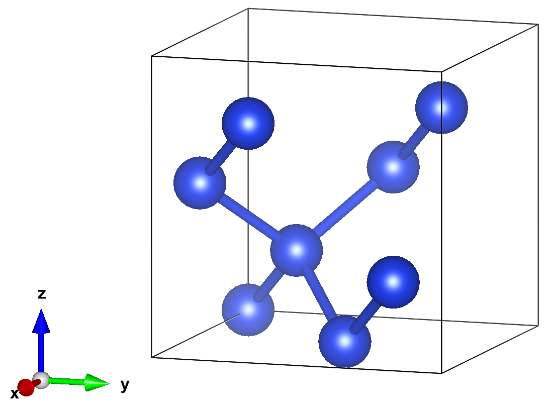
In this example, we will compute the ground state energy and charge density of C diamond in the primitive cell cell.
2.1. DEV TODO#
update image to C primitive cell.
update the following sections to use C / PySCF
“run AFQMC”
“Analyze”
“converge in basis set size”
2.2. External Software#
In addition to SAFIRE and afqmctools, we will be using the following software packages:
PySCF for density functional theory (DFT) calculations, integrals, and some post-processing tools.
VESTA for visualizing the final density.
"""Example of setting up a solids calculation starting
from PySCF.
"""
import h5py
import numpy as np
from pyscf.pbc import gto as pgto
from pyscf.pbc import scf
from mpi4py import MPI

from afqmctools.utils.linalg import get_ortho_ao
from afqmctools.inputs.from_pyscf import pyscf_to_afqmc

### Some parameters for the calculation ###
mesh = (25,)*3  # defines ecut
alat = 3.6  # angstrom
nkx = 2  # kmesh
basis = 'gth-szv'
pseudo = 'gth-pade'
chkfile = 'diamond_2x2x2_rhf.h5'
verbose = 4

rerun = True
###########################################


kpoint_grid_size = (nkx,)*3  # kmesh in 3D

axes = alat/2*np.array([[0, 1, 1],
                        [1, 0, 1],
                        [1, 1, 0]])

atoms = f'''
C 0. 0. 0.0
C {0.25*alat} {0.25*alat} {0.25*alat}
'''

cell = pgto.Cell(
    a = axes,
    atom = atoms,
    basis = basis,
    pseudo = pseudo,
    verbose=verbose,
).build(mesh=mesh)

if rerun:
    kpts = cell.make_kpts(kpoint_grid_size)
    rhf = scf.KRHF(cell, kpts=kpts)
    rhf.chkfile = chkfile
    rhf.run()

    # get and store rotation matrix X to produce orthonormal basis

    X, nmo_per_kpt = get_ortho_ao(rhf.cell, rhf.kpts)

    hcore = rhf.get_hcore()
    fock = hcore+rhf.get_veff()
    # make conversion
    with h5py.File(chkfile, 'a') as fp:
        fp['scf/orthoAORot'] = X
        fp['scf/nmo_per_kpt'] = nmo_per_kpt
        fp['scf/hcore'] = hcore
        fp['scf/fock'] = fock


from pyscf.tools import cubegen
from afqmctools.observables.rhonk import write_gaussian_cube

rdm = rhf.make_rdm1()

nx=ny=nz=50

# the normalization is missing a factor of V / ( nx * ny * nz )
rho = cubegen.density(cell,'diamond_den.cube', rdm, nx=100, ny=100, nz=100)

V = cell.vol
nkpts = len(rhf.kpts)

rho = rho * ( 1 / nkpts ) * ( V / (nx*ny*nz) ) # normalized s.t. $\sum_{\vec{n}} rho_{\vec{n}} = N_{elec} $

data = {
     "axes": np.diag((1.0, 1.0, 1.0)),
     "data": np.random.rand(10, 10, 10), # Volumetric data!
     "elem": [6, 6],
     "pos": [(0, 0, 0), (1, 1, 1)],
     "origin": (0, 0, 0),
     "two_line_comment": "This is a test cube file\nGenerated by write_gaussian_cube\n"
}

write_gaussian_cube("diamond_den_afqmctools.cube",rho)

ngrids = nx*ny*nz

print(f"Integrated charge = {np.sum(rho)}")
print(f"Number of grid points = {ngrids}")
print(f"Charge per grid point = {np.sum(rho)/ngrids}")
2.3. Run AFQMC#
Next, we’ll run SAFIRE using the Hamiltonian and trial wavefunction that we wrote using CoQuí.
We’ve provided an input file in 3_afqmc for this example.
To learn more about the input file, see Understanding the input file.
The input file assumes that you ran CoQuí within the 2_hamiltonian_coqui directory.
If you ran it elsewhere, you will need to update the path to the HDF5 file
in wavefunction accordingly
A key part of the input file is the “estimator” block for the back-propagation algorithm.
"estimator": {
    "name":"back_propagation",
    "path_restoration":true,
    "extra_path_restoration":true,
    "ortho":10,
    "nsteps":400,
    "naverages" : 2,
    "equil":400,
    "onerdm" : {
        "name":"onerdm"
    }
},
The “name” parameter tells SAFIRE what kind of estimator to use ("back_propagation" in this case).
The “nsteps” parameter determines the number of back propagation steps to use.
To check for convergence in the number of back propagation steps, SAFIRE allows multiple “averages” to be set up which each use a different number of steps.
This feature is controlled by setting "naverages" to a value greater than one.
The number of steps that will be used in each average is given by,
where \(a\) is the 0-based index of the “average”, and “nsteps” and “naverages” are corresponding values from the input file. So, for the example here,
and
Now we can run SAFIRE using this input file. We provided a sample Slurm script. In practice, the slurm details will depend on your specific cluster.
#!/bin/bash -l
#SBATCH -J afqmc
#! Number of MPI ranks (= tasks for Slurm)
#SBATCH --ntasks=192
#SBATCH --time=2:00:00

# set up your enviornment as needed here
#
# source /path/to/env.sh

# Launch MPI code...
date
srun --cpu-bind=cores /path/to/safire afqmc.json &> afqmc.out
date
Or, you can run locally with,
$ mpirun -np [number of processes] /path/to/safire afqmc.json &> afqmc.out &
where [number of processes] depends on how many tasks can be run on your local machine.
We’ve included some of the output below. You should see similar numbers in your output.
****************************************************
               Initializing Hamiltonian

****************************************************

 Hamiltonian Factory input:
system: sysid_2
filename: ../2_hamiltonian_coqui/hamiltonian.h5
name: hamiltonian_unique_id_5

 Initializing Hamiltonian from file: ../2_hamiltonian_coqui/hamiltonian.h5
 Found hamiltonian with format: coqui

 - Nuclear coulomb energy: (0.000000, 0.000000)
 - Frozen Core energy: (0.000000, 0.000000)
 - Electron self-interaction energy: (-8.846596, 0.000000)

KPFactorizedHamiltonian input:
name: hamiltonian_unique_id_5
filename: ../2_hamiltonian_coqui/hamiltonian.h5
batched: false
out_of_core: false
cutoff_cholesky: 9.9999999999999995e-07
memory: 4096
nsampleQ: -1


****************************************************
               Initializing Wavefunction

****************************************************
 Wavefunction type: NOMSD
 - Number of determinants in trial wavefunction: 1
 - Coefficient of first determinant: (1.000000, 0.000000)
 getHamOps from scratch
 nkpts: 1

NOMSD input:
nbatch: 0
number_of_references: -1
rediag: false


****************************************************
               Initializing Propagator

****************************************************

BasePropagator input:

nbatch: 0
nbatch_qr: 0
i: -1
a: -1
vbias_bound: 50
external_field_scale: 1
upper_cutoff_scale: 10
lower_cutoff_scale: 1
apply_constrain: true
importance_sampling: true
substractMF: true
hybrid: true
printP1eigval: false
free_projection: false
denseP1: false
external_field:
excited:
debug_verbosity: false


 --------------- Constructing Propagator ------------------

 Using sequential propagation.
 vbias_bound: 50
 Using sparse 1-body propagator
 Using hybrid method to calculate the weights during the propagation.
 Local Energy of starting determinant
  - Total energy    : (-1.191595, 0.000000)
  - One-body energy : (0.800315, 0.000000)
  - Coulomb energy  : (2.632165, 0.000000)
  - Exchange energy : (-4.624075, 0.000000)
When SAFIRE has finished running, you should see the qmc.s000.scalar.dat, and qmc.s000.stat.h5 output data files.
$ ls 3_afqmc
afqmc.json  afqmc.out  qmc.s000.scalar.dat  qmc.s000.stat.h5
2.4. Analyze#
2.4.1. Ground state energy#
afqmctools includes a command line tool for analyzing the scalar data output.
Fun the following command.
If you are running locally, the -t option will cause a plot of the scalar data samples versus total projection time to be generated as seen below.
If you are running remotely, you can add the --savefig [filename].png option to save the figure.
Note, you must still use -t to generate the plot.
!scalar_stats 3_afqmc/qmc.s000.scalar.dat -s time -t -e 5.0 --savefig 3_afqmc/energy_vs_beta.png
Your plot should look similar to the following.
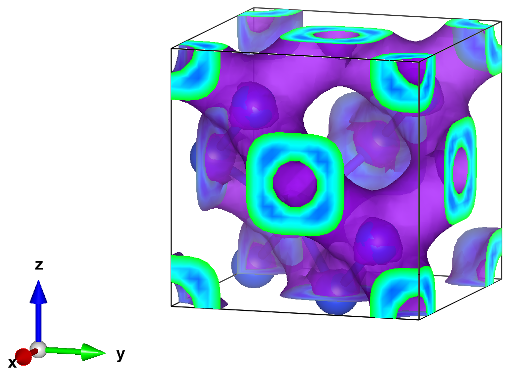
2.4.2. Charge Density#
afqmctools provides a function for generating the real-space charge density
given the one-body reduced density matrix (1rdm), and its stochastic uncertainty from AFQMC, as well as the orbitals from Quantum Espresso.
It will output the resulting 1rdm in a standard *.cube file.
The *.cube file can then be opened in one of several
software packages.
The provided script analysis.py demonstrates how to call the charge_density() function.
from pathlib import Path

from afqmctools.analysis.rdm import average_afqmc_rdm
from afqmctools.observables.rhonk import charge_density

qe_output = Path("./1_dft_quantum_espresso/OUT")
afqmc_path = Path("./3_afqmc")

mean_rdms,err_rdms = average_afqmc_rdm(rdm_file=afqmc_path / "qmc.s000.stat.h5")

num_avgs = mean_rdms.shape[0]
for i in range(num_avgs):
    charge_density(
        mean_rdms[i],
        err_rdms[i],
        orbital_source=qe_output,
        rho_outfile=f"rho_avg{i}_qe_orbs.cube"
    )
Finally, we can open the charge density for visualization. Here we used Vesta to make the following isosurface plot (using an isosurface value of 0.0023)
2.5. Converging in the basis set size#
Accurately capturing electron correlation effects requires a large basis. Here, we are working the basis of Kohn-Sham bands. We will now converge the AFQMC ground state energy, and the charge density in the number of bands used to form the basis,\(N_{bands}\). We have already seen how to perform each step individually above; We will simply need to run AFQMC for a few choices of \(N_{bands}\).
As \(E_\mathrm{AFQMC}\) and \(\rho_\mathrm{AFQMC}(\vec{r})\) begin to converge, each additional band will individually make only a small contribution. It can be useful, then, to choose a logarithmic set of \(\N_{bands}\) to actually run AFQMC for. For example,
>> nbands_log = [ 20*(2**p) for p in range(6) ]
>>> nbands_log
[20, 40, 80, 160, 320, 640]
would allow you to see large changes between each successive run. More points can be added in between these if needed.
DEV TODO: add in results form this.