4. Vanadium Atom (Fully Polarized)#

This example demonstrates a fully polarized AFQMC calculation on an isolated vanadium atom which has a ground state with \(S=3/2\) (quartet state). We will use the frozen core approximation to freeze all electrons except for the \(3d^3\) valence electrons. In the cc-pVDZ basis set, this results in 32 active orbitals and 3 active electrons. We will use CASCI to compute the exact energy within the active space as a reference for comparison with AFQMC.

4.1. Running the Example#

The workflow follows three steps:

Generate an orbital basis: Execute scf/scf.py to perform ROHF on the vanadium atom which we will use as a basis, and to generate a trial wavefunction for AFQMC. We also run a CASCI(32o,3e) calculation to provide a reference energy.

The ROHF energy should be around -942.873080272797 Ha, and the CASCI(32o,3e) energy should be around -942.901099297148 Ha where the contribution in the active space is -3.53263111527235 Ha.
Create AFQMC inputs: Execute input/setup.py to generate the SAFIRE inputs. Note that script uses an active space for AFQMC of cas_afqmc = (3,32). This treats the system as having all electrons in the spin-up channel. The script writes both the Hamiltonian and a fully polarized trial wavefunction to afqmc.h5.
Run SAFIRE: Execute SAFIRE using the provided afqmc.json input file:

First, go to the inputs directory, then run SAFIRE with the following command:
```
mpirun -n 64 safire afqmc.json
```
SAFIRE will use fully polarized walkers, which is computationally efficient for systems with only one spin channel containing all electrons.

analyze the results: Use the scalar_stats command-line tool from afqmctools to analyze the energy output:

$ scalar_stats qmc.s000.scalar.dat -s time -e 5.0 -t --savefig energy_vs_beta.png

====== [analyze_scalar_data Settings] ======

[+] fname            = qmc.s000.scalar.dat
[+] mark_header      = #
[+] series_column    = time
[+] nequil           = 5.0
[+] estimate_equil   = False
[+] column           = LocalEnergy
[+] reblock          = 1
[+] ndiscard         = None
[+] list             = False
[+] trace            = True
[+] append           = None
[+] dump             = False
[+] dump_fname       = trace.dat
[+] verbose          = True
[+] autocorr         = None
[+] savefig          = energy_vs_beta.png
[+] dump_avail_columns = False

AFQMC Energy   -942.901682 +/-   0.000151 32.25  5.0/35.0

This will compute the average AFQMC energy and stochastic uncertainty, using an equilibration time of 5.0 Ha^{-1}. The -t flag will generate a plot of the energy as a function of imaginary time if running locally. If running remotely, you can save the plot of the energy vs imaginary time to a file using the –savefig [name].png option. In either case, you should see the following output if you used the same settings as in the provided afqmc.json file and above.

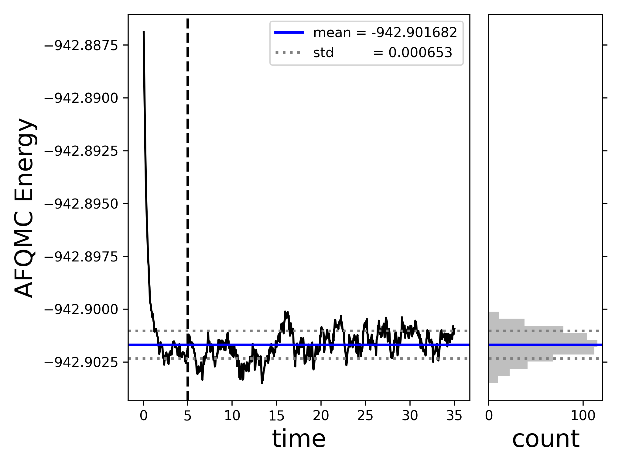
compare with the reference CASCI energy: The AFQMC energy, -942.9017(2) Ha, agrees with the CASCI energy, -942.902141 Ha, which is the exact energy within the active space, to well within chemical accuracy.

See run.sh for execution details. The dice/ directory contains an alternative trial wavefunction generation approach using selected CI.

4.2. Files#

SCF/CASCI Calculation (scf/scf.py):

#!/usr/bin/env python3

# This file is distributed under the Apache License, Version 2.0 License.
# See LICENSE file in top directory for details.
#
# Copyright (c) 2021-2025 The Simons Foundation, Inc.
#
# You may not use this file except in compliance with the License.
# You may obtain a copy of the License at
#
#      http://www.apache.org/licenses/LICENSE-2.0

import numpy as np
import matplotlib.pyplot as plt
from pyscf import gto, scf, mcscf


def main():
    """
    Computing the energy of ferro-magnetically coupled
       Vandium atoms.
    """

    # 0. use an isolated vanadium atom to build a guess for the ferro-magnetic case
    single_mol = gto.M(
        atom='V 0. 0. 0.',
        basis='ccpvdz',
        spin=3,
        verbose=5
    )

    # this will be a basis
    mf = scf.ROHF(single_mol).newton()
    mf.chkfile = 'rohf.chk'
    mf.kernel()

    # Report ROHF energy decomposition and total energy.
    e_elec, e_coul = mf.energy_elec()
    e_nuc = mf.energy_nuc()
    e_one = e_elec - e_coul
    e_tot = mf.e_tot

    print("ROHF one-electron energy: ", e_one)
    print("ROHF Coulomb/exchange energy: ", e_coul)
    print("ROHF electronic energy: ", e_elec)
    print("ROHF nuclear repulsion energy: ", e_nuc)
    print("ROHF total energy: ", e_tot)

    
    
    # Getting a reference energy:
    mycas = mcscf.CASCI(mf,32,3)
    E_casci =  mycas.kernel()
    print("CASCI(32,3) energy: ", E_casci[0])


if __name__ == '__main__':
    main()

Hamiltonian Generation (input/setup.py):