
Download this notebook (.ipynb + data files)
2. Stripes and the square Hubbard Model#
Author: Ryan Levy
import os
# This are in case you have a GPU enabled JAX but are running on CPU.
os.environ['JAX_PLATFORMS'] = 'cpu'
# If you want to use GPU enabled Jax in multiply notebooks with the same
os.environ["XLA_PYTHON_CLIENT_PREALLOCATE"] = "false"

# use x64 numbers
from jax import config
config.update("jax_enable_x64", True)
import matplotlib.pyplot as plt
import numpy as np

import afqmctools.systems.lattice as lat
import afqmctools.utils.visualize as vis
import afqmctools.utils.io as io
import afqmctools.hamiltonian.model.director as ham

from afqmctools.wavefunction.converter import read_wavefunction
from afqmctools.wavefunction.model import write_free_electron_wfn
from afqmctools.analysis.rdm import average_afqmc_rdm

from afqmctools.observables.greens import greens_1body
import afqmctools.observables.spin as spobs
from afqmctools.inputs.from_autohf import autohf_to_afqmc

from tutorial_utils import run_afqmc

import autohf

from pathlib import Path
scratch_dir = Path("data")
scratch_dir.mkdir(parents=True, exist_ok=True)
2.1. Physics Background#
In the paper Stripes and spin-density waves in the doped two-dimensional Hubbard model: Ground state phase diagram [1] we see that for the nearest-neighbor square Hubbard model, the ground state may have a stable staggered stripe ground state order
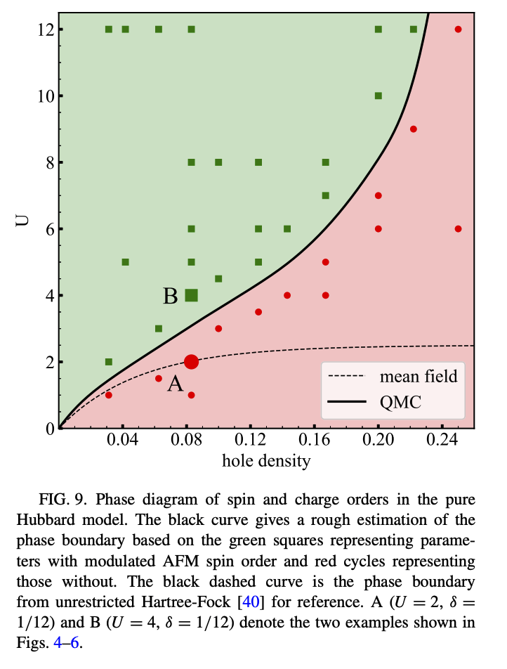
We’ll explore how to see this with AFQMC and the role of the trial wave function
[1] Hao Xu, Hao Shi, Ettore Vitali, Mingpu Qin, and Shiwei Zhang Phys. Rev. Research 4, 013239 – Published 28 March 2022
2.2. Obtaining the Spin density#
Let’s look at a 10x4 system with 0.2 doping at \(U=6\) with a staggered AFM pinning field at the edges. The pinning breaks symmetry in order to understand the response of the system to the applied field.
When confronted with a new problem, the first thing we generally do is use a non-interacting (free electron) wave function as the trial. Let’s do that now
U = 6.0
lattice_dims = (10,4)

lattice_params = {
    'L1' : lattice_dims[0],
    'L2' : lattice_dims[1],
    'boundary1' : 'Open',
    'boundary2' : 'PBC'
}

import afqmctools.systems.lattice as lat

lattice = lat.get_lattice(params=lattice_params)

Ne = int(lattice.N_sites*(1-0.2))//2
nelec = (Ne,Ne)
nelec
vis.plot_lattice(lattice)
The Hamiltonian will be simple,
and we have a convenience function to add the edge pinning as well. We’ll assume \(t=1\), \(h_i=0.5\) just like in the paper
builder = ham.HamiltonianBuilder(
          lattice=lattice,
          spin_symm="collinear" # we have no spin-flip terms
)
# add standard Hubbard terms
builder.nth_neighbor_hopping(1.0)
builder.onsite_hubbard(U)
builder.afm_pinning(0.5)
builder.finalize()
io.write_model_hamiltonian(builder.hamiltonian, scratch_dir / "afqmc.h5",
                        nelec=nelec,spin_symm="collinear")
# get a trial wavefunction: First, let's try a free-electron (i.e. non-interacting) wavefunction
from afqmctools.wavefunction.model import write_free_electron_wfn
write_free_electron_wfn(
    hamiltonian_fname=scratch_dir / "afqmc.h5",
    nelec=nelec
)
Now we’ll write the file to run AFQMC. There are some better tools than this but let’s hard code some things for now
from afqmctools.inputs.from_hdf import write_json

# make an input file
afqmc_params = {
        "timestep": 0.005,
        "steps": 10000,
        "population_control_interval": 2,
        "walker_ortho_interval": 2,
        "n_walkers_per_mpi_task": 40,
        "measure_interval_multiplier": 1,
        "estimator1": {
            "name": "energy",
            "overwrite": True,
            "print_components": True
        },
        "estimator2": {
            "name":"back_propagation",
            "path_restoration": True,
            "extra_path_restoration": True,
            "bp_walker_ortho_interval": 2,
            "measure_interval_multiplier": 250,
            "equil_multiplier": 1000,
            "onerdm" : {
                "name":"onerdm"
    	    }
        },
        "seed" : 42,                          # just for reproducibility
        "propagator": {
            "use_cp_constraint": True,
            "use_real_vbias" : True
        }
    }

write_json(
    scratch_dir / "afqmc.json",
    fwfn0=scratch_dir / "afqmc.h5",
    fham0=scratch_dir / "afqmc.h5",
    exec_opts=afqmc_params,
    series=0
)
!cd data; mpirun -np 16 $AFQMC_EXEC afqmc.json
# analyze
from stats.scalar_dat import analyze_scalar_data

nequil = 20.0

analysis_settings = dict(
    fname = scratch_dir / "qmc.s000.scalar.dat",
    xaxis = "time",     # use units of imaginary time for equilibration
    nequil = 5,    # length of equilibration phase (in units of imaginary time)
    trace = True,       # plots a trace of the scalar data
)

E,dE = analyze_scalar_data(analysis_settings)
2.2.1. Analysis#
We’ll now analyze the spin density of the output given the free electron trial
def staggeredSigns(Nx,Ny):
  signs = np.concatenate([(-1)**(np.arange(Nx)+1),(-1)**(np.arange(Nx))]*(Ny//2)).reshape(Ny,Nx).T.flatten()
  return -signs

def averageOverCols(Sz,Nx,Ny):
    return (Sz*staggeredSigns(*lattice.L)).reshape(*lattice_dims).mean(1)
rho_avg, delta_rho = average_afqmc_rdm(rdm_file=scratch_dir / "qmc.s000.stat.h5")
Xs,Ys,Zs = spobs.local_spin(np.vstack(rho_avg[0]),"collinear").real

delta_Sz = np.sqrt(delta_rho[0,0].diagonal()**2+delta_rho[0,1].diagonal()**2 )
# We're collinear
assert np.allclose(Xs,0)
assert np.allclose(Ys,0)
plt.imshow(Zs.reshape(*lattice.L).T)
plt.colorbar()
plt.show()

plt.imshow(delta_Sz.reshape(*lattice.L).T)
plt.colorbar()
plt.show()
# DMRG data of the form: site Sz Nup Ndn
SzDmrg = np.loadtxt("data_10x4_Ne16U6.0_15360.dat",usecols=(1,))
# now we'll average over the columns

avg_delta_Sz = np.sqrt((delta_Sz.reshape(*lattice.L)**2).sum(1)) / lattice.L[1]

plt.errorbar(np.arange(lattice.L[0]),averageOverCols(Zs,*lattice.L),yerr=avg_delta_Sz,
             fmt='o-',label="AFQMC Free Electron")
plt.plot(-averageOverCols(SzDmrg,*lattice.L),label="DMRG",c='k')

plt.xlabel("Col")
plt.ylabel("Staggered Sz")
plt.legend()

# plt.ylim(-0.3,0.2)
plt.show()
2.3. Self Consistency w/ Hartree-Fock#
The idea behind self-consistent AFQMC is to have the trial wave function match as much as possible the output of AFQMC.
For this model, we can do this by introducing an effective Hubbard model, where \(U\) is replaced with \(U_\text{eff}\). By solving Hartree-Fock (mean field theory) for this effective model and using the result as a trial wave function, we can scan through different \(U_\text{eff}\) to find the one that matches the best.
We’ll use AutoHF to explore creating a trial wave function for AFQMC. Let’s do a few between \(U_\text{eff}=1\) and \(U_\text{eff}=4\)
Note: The Hartree-Fock code is faster if you use a GPU
Ueffs = [1,2,3,4]
for Ueff in Ueffs:

    builder_eff = ham.HamiltonianBuilder(
              lattice=lattice,
              spin_symm="collinear"
                  )
    # add standard Hubbard terms
    builder_eff.nth_neighbor_hopping(1.0)
    builder_eff.onsite_hubbard(Ueff) # We want our HF solver to solve Ueff not U
    builder_eff.afm_pinning(0.5)
    builder_eff.finalize()

    # NOTICE: we must be careful here! We can either keep around afqmc.h5
    # which has the original Hamiltonian (U=6) and keep the wf and its Hamiltonian together
    # or we have one file with afqmc_Ueff which has both the wf and builder.hamiltonian
    io.write_model_hamiltonian(builder_eff.hamiltonian, scratch_dir / f"afqmc_{Ueff}.h5",
                            nelec=nelec,spin_symm="collinear")

    hf_settings = dict(
        steps = 2000,
        opt_method="lbfgs",
        ansatz="SD_ROT",
        nelec = nelec,
        batch_size = 8,
        seed = 1,
        noncollinear = False
    )
    results = autohf.solver.lattice_hf(
        hamiltonian=autohf.AutoHFHamiltonian(builder_eff.hamiltonian),
        lattice=lattice,
        settings=hf_settings,
    )
    autohf_to_afqmc(
        results,
        output_fname = scratch_dir / f"afqmc_{Ueff}.h5"
    )

    write_json(
        scratch_dir / f"afqmc_{Ueff}.json",
        fwfn0=scratch_dir / f"afqmc_{Ueff}.h5",
        fham0=scratch_dir / "afqmc.h5",
        exec_opts=afqmc_params,
        id = f"afqmc_{Ueff}"
    )
    print(f"Written {Ueff}")
for Ueff in Ueffs:
    run_afqmc(
        run_dir = scratch_dir,
        input_file = f"afqmc_{Ueff}.json",
        np = 16,
        output_file = None
    )
rhos, deltas = [],[]

for Ueff in Ueffs:
    if Ueff==0:
        fname = "qmc.s000.stat.h5"
    else:
        fname = f"afqmc_{Ueff}.s000.stat.h5"
    rho_avg, delta_rho = average_afqmc_rdm(rdm_file=scratch_dir / fname)
    rhos.append(rho_avg)
    deltas.append(delta_rho)
for Ueff,rho_avg,delta_rho in zip(Ueffs,rhos,deltas):
    Xs,Ys,Zs = spobs.local_spin(np.vstack(rho_avg[0]),"collinear").real

    delta_Sz = np.sqrt(delta_rho[0,0].diagonal()**2+delta_rho[0,1].diagonal()**2 )
    # We're collinear
    assert np.allclose(Xs,0)
    assert np.allclose(Ys,0)

    fig,axes = plt.subplots(1,2,figsize=(12,4))
    p = axes[0].matshow(Zs.reshape(*lattice.L).T)
    plt.colorbar(p,ax= axes[0], label = "$S^z$")


    p =axes[1].matshow(delta_Sz.reshape(*lattice.L).T)
    plt.colorbar(p,ax= axes[1], label="$ΔSz$")
    if Ueff==0:
        fig.suptitle(f"Free Electron")
    else:
        fig.suptitle(f"{Ueff=}")
    plt.show()
2.4. Self-Consistent Condition#
We’ll now measure the error between the trial wave function’s observable and the output from AFQMC
trial_rhos = []
for Ueff in Ueffs:
    if Ueff==0:
        fname = "afqmc.h5"
    else:
        fname = f"afqmc_{Ueff}.h5"
    (coeffs,wfn), psi0, (na, nb),spintype = read_wavefunction(scratch_dir / fname)
    # We assume spin balance below
    o = wfn.reshape(lattice.N_sites,na,2,order='F').real
    o = np.stack([o[:,:,0],o[:,:,1]])

    rdm = greens_1body(o)
    trial_rhos.append(rdm)
# now we'll average over the columns
for Ueff,rho in zip(Ueffs,rhos):
    Xs,Ys,Zs = spobs.local_spin(np.vstack(rho[0]),"collinear").real

    avg_delta_Sz = np.sqrt((delta_Sz.reshape(*lattice.L)**2).sum(1)) / lattice.L[1]
    if Ueff==0:
        label = "Free Electron"
    else:
        label = f"HF W/ HF Ueff={Ueff}"

    plt.errorbar(np.arange(lattice.L[0]),
                 averageOverCols(Zs,*lattice.L),yerr=avg_delta_Sz,
                 fmt='o--',label=label)
plt.plot(-averageOverCols(SzDmrg,*lattice.L),'x-',label="DMRG",c='k')

plt.xlabel("Col")
plt.ylabel("Staggered Sz")
plt.legend()

# plt.ylim(-0.3,0.2)
plt.show()
Ueffs = [0,1,2,3,4]

dmrg_sz = -averageOverCols(SzDmrg,*lattice.L)

xs,ys,yerrs = [],[],[]
for Ueff,rho_avg,delta_rho,trial_rho in zip(Ueffs,rhos,deltas,trial_rhos):
    XsT,YsT,ZsT = spobs.local_spin(np.vstack(trial_rho),"collinear").real
    Xs,Ys,Zs = spobs.local_spin(np.vstack(rho_avg[0]),"collinear").real

    afqmc_sz = averageOverCols(Zs,*lattice.L)
    trial_sz = averageOverCols(ZsT,*lattice.L)


    delta_Sz = np.sqrt(delta_rho[0,0].diagonal()**2+delta_rho[0,1].diagonal()**2 )
    avg_delta_Sz = np.sqrt((delta_Sz.reshape(*lattice.L)**2).sum(1)) / lattice.L[1]

    xs.append(Ueff)
    ys.append(np.mean(np.abs(afqmc_sz-dmrg_sz)))
    yerrs.append(np.mean(avg_delta_Sz**2))

plt.errorbar(xs,ys,yerr=yerrs,fmt='o-',label="AFQMC",capsize=6)
plt.xticks(Ueffs)
plt.xlabel("Ueff")
plt.ylabel(r"$\langle |$DMRG $S_z - $AFQMC $S_z|\rangle$",fontsize=12)
plt.legend()
plt.grid()

# plt.ylim(-0.3,0.2)
plt.show()


xs,ys,yerrs = [],[],[]
for Ueff,rho_avg,delta_rho,trial_rho in zip(Ueffs,rhos,deltas,trial_rhos):
    XsT,YsT,ZsT = spobs.local_spin(np.vstack(trial_rho),"collinear").real
    Xs,Ys,Zs = spobs.local_spin(np.vstack(rho_avg[0]),"collinear").real

    afqmc_sz = averageOverCols(Zs,*lattice.L)
    trial_sz = averageOverCols(ZsT,*lattice.L)


    delta_Sz = np.sqrt(delta_rho[0,0].diagonal()**2+delta_rho[0,1].diagonal()**2 )
    avg_delta_Sz = np.sqrt((delta_Sz.reshape(*lattice.L)**2).sum(1)) / lattice.L[1]

    xs.append(Ueff)
    ys.append(np.mean(np.abs(afqmc_sz-trial_sz)))
    yerrs.append(np.mean(avg_delta_Sz**2))

plt.errorbar(xs,ys,yerr=yerrs,fmt='o-',label="AFQMC",capsize=6)
plt.xticks(Ueffs)
plt.xlabel("Ueff")
plt.ylabel(r"$\langle |$Trial $S_z - $AFQMC $S_z|\rangle$",fontsize=12)
plt.legend()
plt.grid()

# plt.ylim(-0.3,0.2)
plt.show()
So we can see that somewhere around \(U_\text{eff}\approx 3\) would have the lowest error for self consistency. Despite the difference between DMRG and AFQMC being on average 0.01, there is a clear optimal trial wave function to use. For fine tuning between \(U_\text{eff}\in [2,4]\), we’ll need more sophisticated methods than presented here.
In our original study, we found the optimal \(U_\text{eff} \approx 2.77\)
2.5. Your Turn#
2.5.1. Part 1 – Recreate Fig 1.#
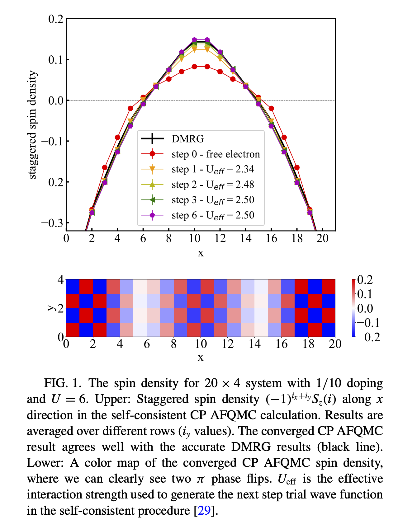
Let’s recreate figure 1 from Xu et al, by changing
Lattice size 10 × 4 to 20 × 4
Doping 0.2 to 0.1 hole doping
\(U = 6\) ✓
2.5.2. Part 2 - Try different settings#
Lets use this as a test bed to explore how AFQMC responds to different settings. Some questions to consider
Use \(U_\text{eff} = U\) or the “bare U” Hartree-Fock trial. How does the quality of the results change?
We compared spin densities, what about hole density? This is the effectively the same as comparing charge density.
Use a trial with a small number of steps so that the solver doesn’t converge. How do the results change? How could you tell this trial isn’t good?
The free electron trial isn’t a valid RHF state (why?). What would be the corresponding RHF solution? What does that output look like?
Explore the parameters of backpropagation, how does the 1rdm change as a function of
nsteps? you can includenaveragesto see the results converge