
Download this notebook (.ipynb + data files)
3. Momentum Distribution of Solid Na#
In this example, we compute the valence momentum distribution \(n(\mathbf{q})\) of bcc sodium with back-propagated AFQMC and compare it with the Compton-scattering experiment and DMC of Huotari et al., Phys. Rev. Lett. 105, 086403 (2010).
3.1. System#
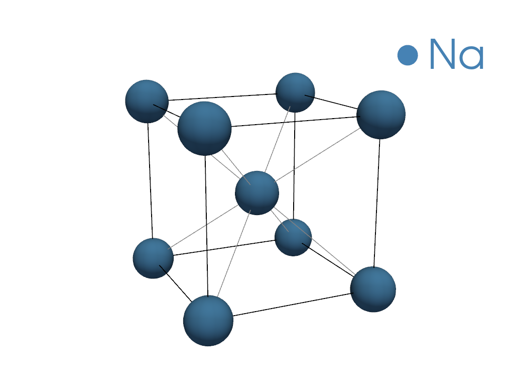
We use the 2-atom cubic cell of bcc Na at the density of the experiment, \(r_s = 3.99\), which gives \(a = 8.1036\) Bohr (4.288 Å). The ccECP pseudopotential has a Ne core, so each atom has 1 valence electron. A \(3\times3\times3\) k-point mesh makes the AFQMC supercell 54 atoms with 54 electrons, which fill the free-electron shells 1 + 6 + 12 + 8 per spin exactly.
3.2. Momentum Distribution from the One-Body Density Matrix#
SAFIRE measures the one-body density matrix in the basis of Kohn-Sham Bloch orbitals, \(\rho_{ij}(\mathbf{k}) = \langle c^\dagger_{i\mathbf{k}} c_{j\mathbf{k}} \rangle\), which is block-diagonal in \(\mathbf{k}\). Expanding each orbital in plane waves, \(\psi_{i\mathbf{k}}(\mathbf{r}) \propto \sum_\mathbf{G} c_{i\mathbf{k}}(\mathbf{G})\, e^{i(\mathbf{k}+\mathbf{G})\cdot\mathbf{r}}\), gives the occupation of momentum \(\mathbf{q} = \mathbf{k}+\mathbf{G}\):
The density matrix does not commute with the Hamiltonian, so we use the back-propagated estimator
(see Computing General Observables).
The plane-wave coefficients come from the QE wavefunction files, and files/nq_tools.py does the unfolding.
Set QE_BIN to the directory holding pw.x and pw2coqui.x, and COQUI_EXEC and AFQMC_EXEC to the
CoQuí and SAFIRE executables.
import csv
import shutil
from pathlib import Path

import h5py
import matplotlib.pyplot as plt
import numpy as np
from safiretools import Results, Wavefunction, write_jobfile

from files.nq_tools import fermi_wavevector, plot_slab, radial_average, read_qe_orbitals, unfold_nq

NP = 12  # MPI ranks
data = Path("data")
for step in ["1_dft_qe", "2_coqui"]:
    shutil.copytree(Path("files") / step, data / step, dirs_exist_ok=True)
(data / "3_safire").mkdir(exist_ok=True)
3.3. Step 1: DFT with Quantum ESPRESSO#
An scf run on an \(8\times8\times8\) mesh gives the density, and an nscf run computes 40 bands on the
\(3\times3\times3\) mesh without symmetry reduction. pw2coqui.x converts the result for CoQuí.
!cd {data}/1_dft_qe && mpirun -n {NP} $$QE_BIN/pw.x -in scf.in > scf.out
!cd {data}/1_dft_qe && mpirun -n {NP} $$QE_BIN/pw.x -in nscf.in > nscf.out
!cd {data}/1_dft_qe && $$QE_BIN/pw2coqui.x -in pw2coqui.in > pw2coqui.out
3.4. Step 2: Hamiltonian and Trial Wavefunction with CoQuí#
CoQuí writes the Hamiltonian in the basis of the lowest 19 bands per k (513 orbitals), with Cholesky-decomposed two-electron integrals, and the Kohn-Sham determinant as the trial wavefunction. 19 bands reach about 19 eV above the Fermi energy without splitting a degenerate level.
!cat {data}/2_coqui/input.toml
!cd {data}/2_coqui && mpirun -n {NP} $$COQUI_EXEC input.toml > coqui.out

with h5py.File(data / "2_coqui/hamiltonian.h5") as f:
    kpoints = f["System/BZ/kpoints"][...]
    volume = abs(np.linalg.det(f["System/lattice_vectors"][...]))
    occ = f["Orbitals/occ"][...]  # Kohn-Sham occupations per spin, (1, nk, M)
nk, M = occ.shape[1:]
k_F = fermi_wavevector(volume, 2)  # 2 valence electrons per cell
print(f"nk = {nk}, NMO = {nk * M}, k_F = {k_F:.4f} Bohr^-1")
3.5. Step 3: Run AFQMC#
CoQuí writes a collinear trial with identical spin determinants. We rebuild it as a closed-shell trial,
so that SAFIRE can use closed-shell walkers, which propagate one spin.
The back-propagated density matrix is measured at each back-propagation length in bp_lengths.
A new window starts every max(bp_lengths) steps after equilibration, so each length gives one sample per window.
alpha, beta = Wavefunction.from_hdf5(data / "2_coqui/wfn.h5").determinant(0)
assert np.allclose(alpha, beta)

bp_lengths = [100, 200]
# bp_lengths = [100, 200, 400, 600] # takes some time
write_jobfile(data / "3_safire/afqmc.json", {
    "seed": 7,
    "execute": {
        "wavefunction": Wavefunction.from_single_determinant(alpha),
        "hamiltonian": {"filename": "../2_coqui/hamiltonian.h5"},
        "timestep": 0.01,
        "steps": 5000,
        "equilibration_steps": 600,
        "measure_interval": 10,
        "population_control_interval": 10,
        "walker_ortho_interval": 10,
        "num_walkers": 40,
        "estimators": {
            "energy": None,
            "backprop": {"propagation_steps": bp_lengths, "onerdm": {}},
        },
    },
})
!cd {data}/3_safire && mpirun -n {NP} $$AFQMC_EXEC afqmc.json
3.6. Step 4: Momentum Distribution#
We unfold the Kohn-Sham occupations for the DFT \(n(\mathbf{q})\), and the back-propagated density matrix inside
Results.evaluate for jackknife error bars on its radial average.
results = Results(data / "3_safire/afqmc.results.h5")

qvecs, coeffs = read_qe_orbitals(data / "1_dft_qe/OUT/pwscf.save", kpoints, M)
qmag = np.linalg.norm(qvecs, axis=1)
edges = np.linspace(0, 2.5 * k_F, 81)
q_bins = radial_average(qmag, qmag, edges)[0]

def radial_nq(rdm):
    return radial_average(qmag, unfold_nq(rdm, coeffs), edges)[1]

n_dft = radial_nq(np.diag(occ.ravel())[None])

bp = {}
for L in bp_lengths:
    bp[L] = results.evaluate(radial_nq, [f"BackPropEstimator/Steps={L}/OneRDM"])
above = np.argmax(q_bins > k_F)  # first radial bin above k_F
print(f"n(q) at |q| = {q_bins[above]:.3f} Bohr^-1: DFT {n_dft[above]:.3f}")
for L, (n, dn) in bp.items():
    print(f"  BP {L:3d}: {n[above]:.3f} +/- {dn[above]:.3f}")
Back propagation moves electrons above \(k_\mathrm{F}\), and the amount still grows with the back-propagation length.
3.7. Comparison with DMC and Experiment#
The experimental and DMC data were extracted from Fig. 1 of Huotari et al. and are per spin, so we divide ours by 2. Our cell has the experimental density, so we compare on absolute momentum.
with open("files/huotari2010_fig1_nofp.csv") as f:
    rows = list(csv.DictReader(line for line in f if not line.startswith("#")))

def huotari(series, *columns):
    return np.array([[float(r[c]) for c in columns] for r in rows if r["series"] == series]).T

max_bp_length = max(bp_lengths)

bp_rdm, _ = results.average(f"BackPropEstimator/Steps={max_bp_length}/OneRDM")

fig, (ax0, ax1) = plt.subplots(1, 2, figsize=(11, 4.5))
plot_slab(ax0, qvecs, unfold_nq(bp_rdm, coeffs) / 2, k_F)
ax0.set_title(ax0.get_title() + f", BP {max_bp_length}")

ax1.plot(q_bins, n_dft / 2, "s", color="0.5", mfc="none", ms=6, label="DFT")
n, dn = bp[max_bp_length]
ax1.errorbar(q_bins, n / 2, yerr=dn / 2, fmt="o", color="C3", ms=4, capsize=2, label=f"AFQMC BP {max_bp_length}")
p, n = huotari("QMC", "p_au", "n")
ax1.plot(p, n, "k-", lw=1.5, label="DMC (Huotari 2010)")
for series, marker, label in [("exp_run1", "s", "experiment, run 1"), ("exp_run2", "^", "experiment, run 2")]:
    p, n, dn = huotari(series, "p_au", "n", "n_err")
    ax1.errorbar(p, n, yerr=dn, fmt=marker, color="C0", mfc="none", ms=5, capsize=2, label=label)
ax1.axvline(k_F, color="0.3", ls=":", lw=1)
ax1.set(xlabel=r"$p$ (a.u.)", ylabel=r"valence $n(p)$ per spin", xlim=(0, 2 * k_F), ylim=(-0.05, 1.05),
        title="Comparison with Huotari et al.")
ax1.grid(alpha=0.3)
ax1.legend(fontsize=8)
fig.tight_layout()
fig.savefig(data / "nq_Na.png", dpi=200)
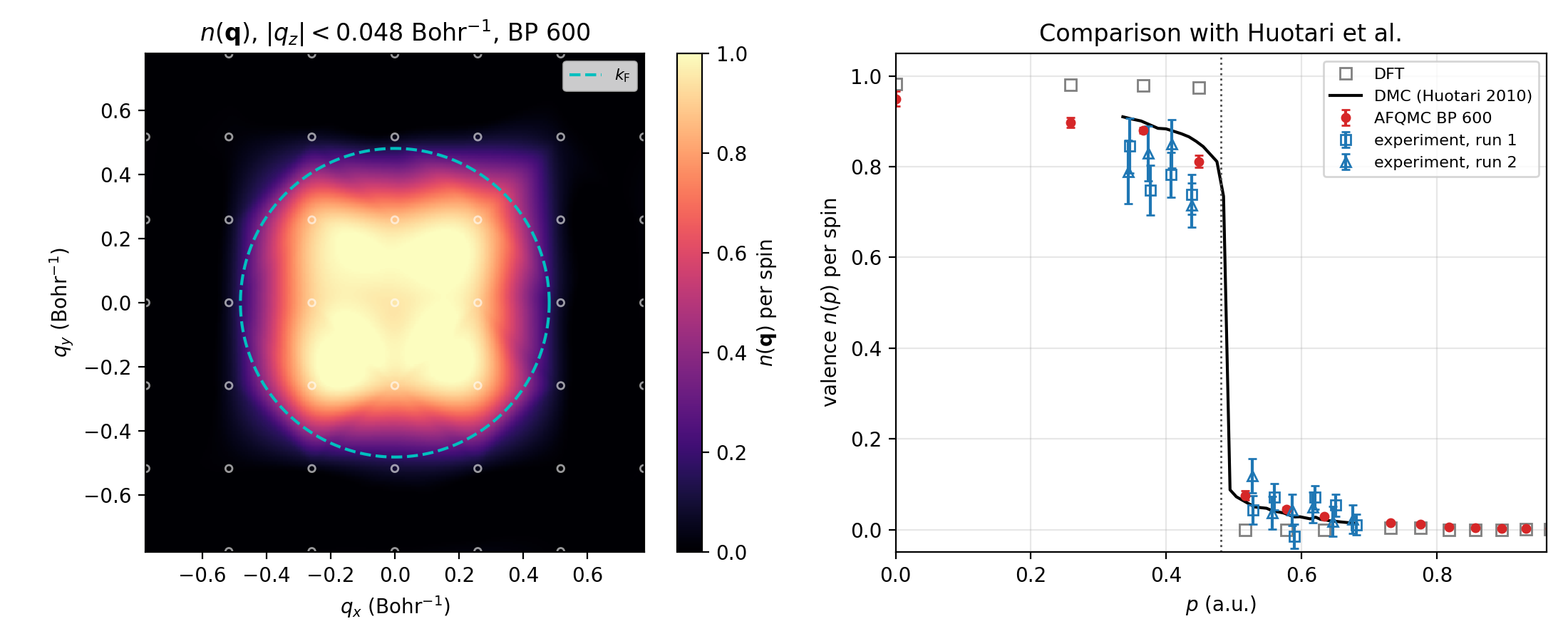
The left panel shows the back-propagated \(n(\mathbf{q})\) per spin in the \(q_z = 0\) plane, with the Fermi sphere dashed. On the right, our points are drawn without connecting lines, because the \(3\times3\times3\) mesh samples only a few shells of \(|\mathbf{q}|\). At \(\tau_\mathrm{BP} = 6\) Ha\(^{-1}\) we obtain good agreement with DMC and experiment, but a production run should converge the back-propagation length, the basis set, the timestep error, and the population control bias.